top of page

For this experiment 2, I will only use the most correlated to target (SalePrice) for the prediction. Moreover, I also skew the target to make the target skew correctly.
ex2: Text
Data Processing
I will use log algorithm to fix the skewness of SalePrice.
ex2: Text

ex2: Image
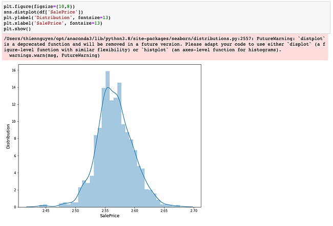
Now, I observe the distribution of SalePrice data to see if our target is now normally skewed or not.
ex2: Text
ex2: Image
Great! Now our target is normally skewed!
ex2: Text
Modeling
I will use the most correlated features to SalePrice to predict our target that is SalePrice. These most correlated features are selected after I observed the correlation between features during the data understanding step above.
ex2: Text

ex2: Image
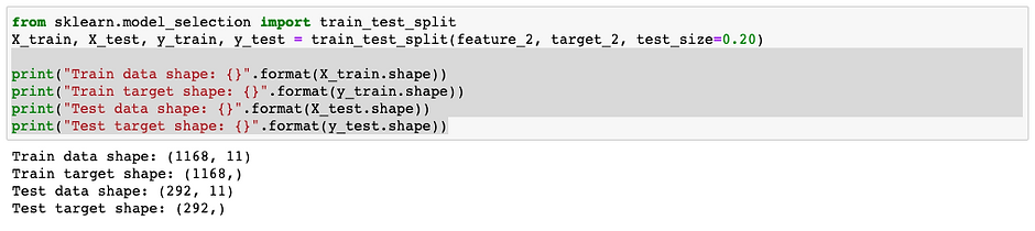
Split the data
ex2: Text
ex2: Image
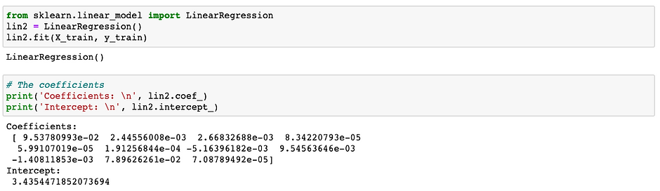
Build and train the model. I will also use the linear regression model for the experiment 2 to be able to draw comparison about how the same model works on this dataset between using all the features and using the most correlated features to the skewed target.
ex2: Text
ex2: Image
Evaluate
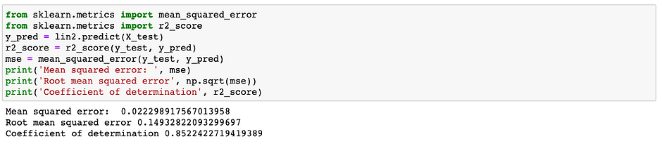
I will also use the MSE and RMSE values and coefficient of determination value to evaluate the performance of my model.
ex2: Text
ex2: Image
Surprisingly, after fixing the skewness of the target (SalePrice) and choosing the most correlated features to the SalePrice, the root mean squared error of linear regression on this dataset now is very small. This means linear regression is the best fit model for this dataset now. Moreover, I also noticed that the coefficient of determination value is also relatively high, which is 0.85. This correlation value means about 85% of the data fit the linear regression model in the experiment 2.
Download my Jupyter Notebook to view my code.
ex2: Text
bottom of page